The example below does not require any additional R packages to be installed (i.e. runs with the basic R installation).
This example conducts power analysis for an expected difference between means equal to 2 with the standard deviation of 1 at a range of alpha and beta values. Any of these four parameters can be estimated when the other three are provided.
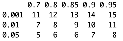
Results are generated as the required sample size to detect expected difference between means at the following alpha (rows) and beta (columns):

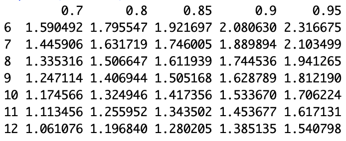
or, as the difference between means that can be detected with the following sample sizes (rows) at alpha=0.05 and beta=0.7-0.95:

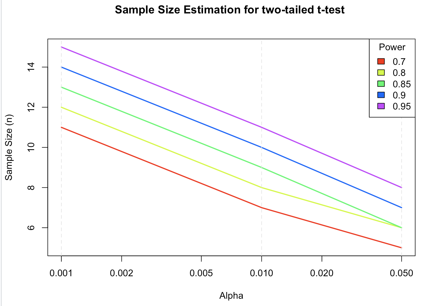
This script also generates a plot summarizing the relationships between all four parameters:

Here is the script:

# calculate sample size required
# to detect expected difference between means
# at the following alpha (0.001, 0.01 and 0.05) and beta (0.7-0.95)

a <- c(.001,.01,.05)
na <- length(a)
p <- c(.7,.8,.85,.9,.95)
np <- length(p)

# d is the expected difference between means
# s is the standard deviation

d <- 2
s <- 1

samsize <- array(numeric(na*np), dim=c(na,np))
for (i in 1:np){
for (j in 1:na){
result <- power.t.test(n = NULL, delta = d, sd = s,
sig.level = a[j], power = p[i],
type = “two.sample”,alternative = “two.sided”)
samsize[j,i] <- ceiling(result$n)
}
}

as.data.frame(samsize)
colnames(samsize) <- p
row.names(samsize) <- a

# calculate difference between means that can be detected
# with the following sample sizes (6 to 12)
# at alpha=0.05 and beta=0.7-0.95

nu <- c(6:12)
nun <- length(nu)

samsize2 <- array(numeric(nun*np), dim=c(nun,np))
for (k in 1:np){
for (m in 1:nun){
result <- power.t.test(n = nu[m], delta = NULL, sd = s,
sig.level = 0.05, power = p[k],
type = “two.sample”,alternative = “two.sided”)
samsize2[m,k] <- result$delta
}
}

as.data.frame(samsize2)
colnames(samsize2) <- p
row.names(samsize2) <- nu

print(samsize)
print(samsize2)

# set up graph

xrange <- range(a)
yrange <- round(range(samsize))
colors <- rainbow(length(p))
plot(xrange, yrange, log=”x”, type=”n”,
xlab=”Alpha”,
ylab=”Sample Size (n)” )

# add power curves

for (i in 1:np){
lines(a, samsize[,i], type=”l”, lwd=2, col=colors[i])
}

# add annotation (grid lines, title, legend)

abline(h=0, v=a, lty=2, col=”grey89″)
title(“Sample Size Estimation for two-tailed t-test \n”)
legend(“topright”, title=”Power”, as.character(p), fill=colors)