We have discussed this topic several times before (HERE and HERE). There seems to be a growing understanding that, when reporting an experiment’s results, one should state clearly what experimental units (biological replicates) are included, and, when applicable, distinguish them from technical replicates.

In discussing this topic with various colleagues, it became obvious to us that there is no clarity on best analytic practices and how to take technical replicates into analysis.

We have approached David L McArthur (at the UCLA Department of Neurosurgery), an expert in study design and analysis, who has been helping us and the Preclinical Data Forum on projects related to data analysis and robust data analysis practices.

A representative example that we wanted to discuss includes 3 treatment groups (labeled A, B, and C) with 6 mice per group and 4 samples processed for each mouse (e.g. one blood draw per mouse separated into four vials and subjected to the same measurement procedure) – i.e. a 3X6X4 dataset.

The text below is based on Dave’s feedback.  Note that Dave is using the term “facet” as an overarching label for anything that contributes to (or fails to contribute to) interpretable coherence beyond background noise in the dataset, and the term “measurement” as a label for the observed value obtained from each sample (rather than the phrase “dependent variable”  often used elsewhere).

Dave has drafted a thought experiment supported by a simulation.  With a simple spreadsheet using only elementary function commands, it’s easy to build a toy study in the form of a flat file representing that 3X6X4 system of data, with the outcome consisting of one measurement in each line of a “tall” datafile, i.e., 72 lines of data with each line having entries for group, subject, sample, and close-but-not-quite-identical measurement (LINK). But, for our purposes, we’ll insert not just measurement A but also measurement B on each line — where we’ve constructed measurement B to differ from measurement A in its variability but otherwise to have identical group means and subject means.  (As shown in Column E, this can be done easily: take each A value, jitter it by uniform application of some multiplier, then subtract out any per-subject mean difference to obtain B.)  With no loss of meaning, in this dataset measurement A has just a little variation from one measurement to the next within a given subject, but because of that multiplier, measurement B has a lot of variation from one measurement to the next within a given subject.

A 14-term descriptive summary shows that using all values of measurement A, across groups, results in:

	a	b	c
N	24.0000	24.0000	24.0000
mean	0.8500	1.4500	2.0500
SD	0.2874	0.2874	0.2874
robust min	0.3000	0.9000	1.5000
min	0.3000	0.9000	1.5000
hdQ: 0.25	0.6380	1.2380	1.8380	… (25th quantile, the lower box bound of a boxplot)
median	0.8500	1.4500	2.0500
hdQ: 0.75	1.0620	1.6620	2.2620	… (75th quantile, the upper box bound of a boxplot)
max	1.4000	2.0000	2.6000
robust max	1.4000	2.0000	2.6000
skew	-0.0000	-0.0000	-0.0000
kurtosis	-0.5908	-0.5908	-0.5908
Huber mu	0.8500	1.4500	2.0500
Shapiro p	0.9703	0.9703	0.9703

while, using all values of  measurement B, across groups, results in:

	a	b	c
N	24.0000	24.0000	24.0000
mean	0.8500	1.4500	2.0500	<– identical group means
SD	5.7131	5.7131	5.7131	<– group standard deviations about 20 times larger
robust min	-6.9000	-6.3000	-5.7000
min	-6.9000	-6.3000	-5.7000
hdQ: 0.25	-4.2657	-3.6657	-3.0657
median	0.8500	1.4500	2.0500	<– identical group medians
hdQ: 0.75	5.9657	6.5657	7.1657
max	8.6000	9.2000	9.8000
robust max	8.6000	9.2000	9.8000
skew	-0.0000	-0.0000	-0.0000	<– identical group skews
kurtosis	-1.3908	-1.3908	-1.3908	<– greater kurtoses, no surprise
Huber mu	0.8500	1.4500	2.0500	<– identical Huber estimates of group centers
Shapiro p	0.0078	0.0078	0.0078	<– suspiciously low p-values for test of normality, no surprise

The left panel in the image below results from simple arithmetical averaging of that dataset’s samples from each subject, with the working dataframe reduced by averaging from 72 lines to 18 lines.  It doesn’t matter here whether we now analyze measurement A or measurement B, as both measurements inside this artificial dataset generate the identical 18-line dataframe, with means of 0.8500, 1.4500, and 2.0500 for groups A, B and C respectively.  Importantly, the sample facet disappears altogether, though we still have group, mouse, measurement and noise.  The simple ANOVA solution for the mean measures shows “very highly significant” differences between the groups.  But wait.

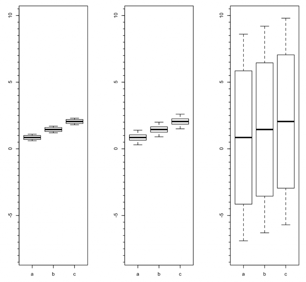
The center panel uses all 72 available datapoints from measurement A.  By definition that’s in the form of a repeated-measures structure, with four non-identical samples provided by each subject.  Mixed effects modeling accounts for all 5 facets here by treating them as fixed (group and sample) or random (subject), or as the object of the equation (measurement), or as residual (noise).  The mixed effects model analysis for measurement A results in “highly significant” differences between groups, though those p-values are not the same as those in the left panel.  But wait.

The right panel uses all 72 available datapoints from measurement B.  Again, it’s a repeated-measures structure, but while the means and medians remain the same, now the standard deviations are 20 times larger than those for measurement A, a feature of the noise facet being intentionally magnified and inserted into the artificial source datafile. The mixed effects model analysis for measurement B results in “not-at-all-close-to-significant” differences between groups; no real surprise.

What does this example teach us?

Averaging technical replicates (as in the left panel) and running statistical analyses on average values means losing potentially important information.  No facet should be dropped from analysis unless one is confident that it can have absolutely no effect on analyses.  A decision to ignore a facet (any facet), drop data and go for a simpler statistical test must in any case be justified and defended.

Further recommendations that are supported by this toy example or that the readers can illustrate for themselves (with the R script LINK) are:

• There is no reason to use the antiquated method of repeated measures ANOVA; in contrast to RM ANOVA, mixed effects modeling makes no sphericity assumption and handles missing data well.
• There is no reason to use nested ANOVA in this context:  nesting is applicable in situations when one or another constraint does not allow crossing every level of one factor with every level of another factor.  In such situations with a nested layout, fewer than all levels of one factor occur within each level of the other factor.  By this definition, the toy example here includes no nesting.
• The expanded descriptive summary can be highly instructive (and is yours to use freely). 

And last but not least, whatever method is used for the analysis, the main message that should be lost – one should be maximally transparent about how the data were collected, what were the experimental units, what were the replicates, and what analyses were used to examine the data.